
An Explanation of Point-Biserial Correlation: Criteria and Application of the Concept
 Introductory statistics textbooks universally present the topic of correlation using the Pearson product-moment correlation coefficient, a formula formalized by Karl Pearson in 1895 a decade after Sir Francis Galton presented the first bivariate scatterplot (Rogers & Nicewander, 1988). The coefficient, an index denoted by r, shows the strength of association between two variables and is a function of raw scores and means.
Although the Pearson product-moment correlation is the most widely used correlation tool, it is not always the most appropriate. There are other types of correlation from which to choose, decisions about which to use determined by the level and type of data and the distribution of that data. One such correlation is the point-biserial correlation rpb which is a special case of the Pearson product-moment correlation. One criterion for the Pearson product-moment correlation is that both variables should be non-dichotomous. Point-biserial correlation, however, is calculated when either the independent variable or dependent variable is dichotomous while the other variable is non-dichotomous.
One Variable Must Be Dichotomous
A dichotomous variable, also known as a binary variable, is one which can be represented by only two values. Often, a dichotomous variable is a categorical variable that is coded 0 or 1. A classic example of a dichotomous categorical variable is gender. The assignation of the value 0 and 1 to female and male categories respectively has nothing to do with a “measurement” of being male or female. That is, 1 does not represent a greater quantity of “gender” or a greater quantity of “maleness.” This can be contrasted with a non-dichotomous variable such as height, where values capture a physical property of a person or object and correspond to greater and lesser quantities of height. Whereas 1 does not represent one more unit of maleness, 1 centimeter represents exactly one more centimeter than zero centimeters.
Gravetter and Wallanau (2009), in Statistics for the Behavioral Sciences, provide some good examples of dichotomous variables:
1. Male versus female
2. College graduate versus not a college graduate
3. First born child versus later-born child
4. Success versus failure on a particular task (p. 548)
In these cases, coding the variable 1 or 0 allows for identification rather than measurement. A person is either male or female, a college graduate or not, a first born or later-born child, and so forth.
In standard correlation, the variables must be interval or ratio level data and consequently non-dichotomous. For example, the correlation between per capita income and the number of medical doctors per 10,000 residents would best be served by the Pearson product-moment correlation, because both variables—income and number of medical doctors—are at the ratio level (differences between measurement values are meaningful and theoretically can be zero). When one of the variables is dichotomous and the other is at the interval or ratio level, then the point-biserial correlation coefficient is a better tool. Although many discussions of the point-biserial correlation assume a dichotomous dependent variable (Y), the independent variable (X) can be dichotomous, as long as the dependent variable is non-dichotomous. (Rosenthal, Rosnow, & Rubin, 2000). In the case where both variables are dichotomous, the phi correlation coefficient is used. For instance, the strength of the relationship between gender and smoking would be better served by phi correlation, instances of smoking or non-smoking coded 0 or 1.
The first step in calculating the point-biserial correlation coefficient is to assign dummy values to the dichotomous variables. Zero and 1 are traditionally used, although one could hypothetically use two other values without affecting the outcome. Instances of the presence of a characteristic are often coded 1 and its absence 0, but this coding is also senstive to how the relationship between variables is conceptualized and how the research hypothesis is phrased. For example, smoking and non-smoking would be coded 1 and 0, respectively, if one hypothesized a positive correlation between smoking and incidence of a particular lung complication. Converesly, if one hypothesized a positive correlation between non-smoking and excercise, non-smoking would be coded 1 and smoking zero.
Calculating the Point-Biserial Correlation Coefficient rpb
The point-biserial correlation coefficient is a special case of the Pearson product-moment correlation; therefore, any standard correlation application or program can be used (e.g., SPSS, SAS, graphing calulator). Vassar, however, has a dedicated point-biserial calculator. If caluclating by hand, the coefficient and can be caluclated using the following forumula:
In reference to the pq notation formula, Mp is the mean for the non-dichotomous values in connection with the variable coded 1, and Mq is the mean for the non-dichotomous values for the same variable coded 0. St is the standard deviation for all non-dichotomous entries, while p and q are the proportion of the dichotomous variable coded 1 and 0, respectively.
Interpreting the Point-Biserial Via the Line of Best Fit
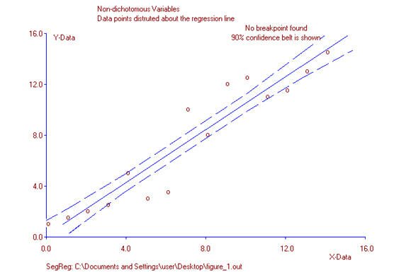
One way to look at the point-biserial correlation is by using the concept of the line of best fit. With the Pearson product-moment correlation, where two variables display some strength of association, data points are distributed about the least squares line. As values of x increase, values for y either increase or decrease along that line. In figure 1, scanning horizontally, it can be seen there are no “large” gaps between data points.
For point-biserial correlation, this characteristic does not hold. Data points will “line up” along the two values of the dichotomous variable with a meaningless gap in between the two columns or rows of data points (figure 2). In figure 2, points are distributed about the least square line only for values 0 and 1. This is because, for the dichotomous variable, any values other than 0 or 1 are undefined, so no data point corresponding to any other value will exist. No data point will be associated with 0.7, for example. For all graphic representations of any given point-biserial correlation, data points will either “line up” vertically or horizontally depending on whether the dichotomous variable is the independent variable (X) or the dependent variable (Y).
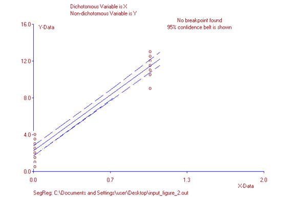
Consequently, the line of best fit does not have any predictive value as in a standard two variable regression model other than at the two values associated with the dichotomous variable. In reference to figure 2, a question such as, “What does the regression line predict for the value of y when x equals 0.7?” is meaningless since there can be no value 0.7 for a variable which can only have only two values: 0 or 1. That is why the concept of a regression model, often discussed in reference to the Pearson r, is not a useful concept when discussing point-biserial correlation.
However, both the Pearson product-moment correlation and the point-biserial correlation measure the strength of association between two variables about the line of best fit. Intuitively speaking, for both types of correlation, the closer the data points as a whole are to the line of best fit, the stronger the correlation. In the case of the point-biserial, the line of best fit passes through the mean values of the non-dichotomous variable associated with each dichotomous variable (assuming the mean values are significantly different). So the closer the non-dichotomous values are to the means for each dichotomous variable, the stronger the correlation will be. Finally, a horizontal or vertical line-of-best fit, depending on whether x or y is the dichotomous variable, will indicate that the means are not significantly different, and as with the Pearson product-moment correlation, will consequently feature a value for rpb at or near zero.
Interpreting the Strength of Association: The Coefficient of Determination
Pett (1997) asserts that the same criteria for evaluating the coefficient of determination in regard to standard correlation can be applied to rpb2 because of the close relationship between rpb and the Pearson r. The coefficient of determination in the form of rpb2, therefore, is a useful index for drawing conclusions from the data. The following intervals for values of r2 apply equally to rpb2.
Very strong: ≥ .81
Strong: .49-.80
Moderate: .25-.48
Weak: .00-.08
As with standard correlation, these ranges function as guidelines rather than absolute indicators of the value of the strength. In some research contexts, a moderate correlation can be very important and be interpreted as “strong.” In other contexts, a correlation between .49 and .80 may not be relevant. It is important to see what the literature indicates about the relationship between variables being studied and how other correlation studies dealing with the same or similar variables interpret the coefficient of determination.
Hypothesis Testing
Even if the coefficient of determination indicates a relationship between variables, the correlation may not be significant. An interpretive index such as the coefficient of determination is not meaningful by itself. It has to be statistically significant. Just because squaring rpb leads to a value of .75 doesn’t necessarily mean the indication of a strong relationship is statistically valid. Perhaps the sample size or correlation is too small in comparison to the other value.
In order to determine if the correlation is significant, the null hypothesis must be rejected. To begin, the null hypothesis always states that rpb equals zero. Any evaluation of a correlation begins with the disprovable statement that there is no correlation between the two variables. Although rarely stated explicitly, the research hypothesis is always formulated with the null hypothesis in mind. If the null hypothesis is rejected, the alternative or research hypothesis can be accepted, namely, rpb is greater or less than zero. Research hypotheses involving the point-biserial correlation will either be positive or negative. For example, Weine et al. (1998) predicted positive association between older age and post-traumatic stress disorder (PSTD) among Bosnia refugees. Older age refugees should show more instances of PTSD. In this case, rpb is greater than zero.
In order to reject the null hypothesis, a t-test for independent means is applied to the correlation coefficient. This is:
![]()
where n is the number of cases, n-2 is the degrees of freedom, and r_pb is the point-biserial correlation coefficient calculated from (1) or a correlation calculator. A one-tailed t-test is used when the correlation is predicted to be either positive or negative. That is, a given research or alternative hypothesis will usually state some variable is positively or negatively related to another variable as opposed to being non-directional.
Using a table or t-statistic calculator, if the value of t obtained is less than the critical value for a one-tailed t-test for independent means associated with the degrees of freedom (n-2) then the null hypothesis cannot be rejected. If the value of t is greater than the critical value associated with the relevant degrees of freedom, then the null hypothesis can be rejected and the research hypothesis supported. Before locating the all-important critical value, the researcher must decide on the level of significance (usually p < .05).
For example, let’s say someone hypothesizes that men prefer watching sports on television compared to women and formulates the hypothesis that being male is positively correlated with a preference for watching sports on television. Based on a sample of 16 participants (8 men and 8 women), this individual found the correlation between gender and preference for watching sports on television to be .40, indicating a moderate correlation. But is this correlation significant? After all, a sample size of n=16 is fairly small. Using the t-statistic, the following t-value obtains:
![]()
The critical value for a correlation value of .40, with 14 degrees of freedom, significant at p <.05 for a one-tailed t-test is 1.76. Because 1.63 is not greater than the critical value, then the null hypothesis cannot be rejected. The researcher’s hypothesis that being male is positively associated with a preference for viewing sports on television compared with being female is not supported.
The researcher’s hypothesis is not disproved. In addition, a contrary conclusion cannot be drawn that there is no preference for sports viewing when comparing men and women or women prefer watching sports. Not supporting a given hypothesis is not the same as disproving it or supporting an opposite hypothesis. In this example, the correlation was indeed positive (.40). The sample size and correlation value, however, may not have been large enough in relation to each other. The research hypothesis may have been supported given a larger sample size. Of course, that is speculative.
A Fictional Example
Let’s apply the ideas above to a fictional example. An urban planner hypothesizes the correlation between lack of car ownership and use of public transportation would be positive in a particular urban location. The planner reasons that those who do not own cars would find more need for public transportation compared to those who own cars and therefore would use public transportation more. The first step in the process of conducting a point-biserial correlation is to figure out what the dichotomous and non-dichotomous variable are. In this case, the dichotomous variable (X) is car ownership, which is the independent variable because it is hypothesized as affecting frequency of public transportation use. The non-dichotomous variable is the number of times in a given time span that person uses public transportation. The non-dichotomous variable is the dependent variable in this example.
Next, the researcher collects a small sample of 18 participants for her study, gathering the following information(Table 1):
| Participant | Car Ownership | Use of Public Transportation |
| 1 | No | 3 |
| 2 | No | 12 |
| 3 | No | 10 |
| 4 | No | 11 |
| 5 | No | 12 |
| 6 | No | 23 |
| 7 | No | 14 |
| 8 | No | 0 |
| 9 | No | 16 |
| 10 | Yes | 0 |
| 11 | Yes | 2 |
| 12 | Yes | 1 |
| 13 | Yes | 0 |
| 14 | Yes | 3 |
| 15 | Yes | 4 |
| 16 | Yes | 0 |
| 17 | Yes | 0 |
| 18 | Yes | 1 |
Table 1. Initial respsonse for 18 participants
A cursory glance at the data reveals that those who do not own a car (participants 1 through 9) have used public transportation more often than those who do own a vehicle (participants 10-18). There appears to be an association between lack of vehicle ownership and the number of times an individual uses public transportation.
The next step would be to code the responses “Yes” as 0 and “No” as 1, making vehicle ownership into a numerically dichotomous variable. At first glance, this may seem counterintuitive because we associate zero as negative response (“no”) and 1 as positive response (“yes”). However, because the researcher hypothesizes the effects of not having a car rather than having a car will be in terms of an increase in public transportation use, the researcher will code “No” responses as 1 as “Yes” responses as 0. Recall that the researcher wants to know about “lack of car ownership,” not car ownership, couching the hypothesis in terms of a positive relationship.
| Participant | Car Ownership | Use of Public Transportation |
| 1 | 1 | 3 |
| 2 | 1 | 12 |
| 3 | 1 | 10 |
| 4 | 1 | 11 |
| 5 | 1 | 12 |
| 6 | 1 | 23 |
| 7 | 1 | 14 |
| 8 | 1 | 0 |
| 9 | 1 | 16 |
| 10 | 0 | 0 |
| 11 | 0 | 2 |
| 12 | 0 | 1 |
| 13 | 0 | 0 |
| 14 | 0 | 3 |
| 15 | 0 | 4 |
| 16 | 0 | 0 |
| 17 | 0 | 0 |
| 18 | 0 | 1 |
Table 2. Yes and no response coded 0 and 1.
Once the qualitative data is coded numerically, the researcher can use the pq formula above to obtain the point-biserial correlation coefficient, namely:
![]()
![]()
Next, the researcher determines whether the coefficient .735 is statistically significant, using a one-tailed t-test as the hypothesis was directional (the prediction was that the relationship between the independent and dependent variables would be positive). The following t-values obtain:
![]()
The critical value corresponding to 16 degrees of freedom, significant at p <.05 for a one-tailed t-test is 1.75. The obtained value (4.34) is greater than 1.75. Therefore, the correlation coefficient is significant. Significance means the results were probably not a result of chance, more likely representing the characteristics of the population from which the sample was drawn, not just the sample itself.
After establishing that the rpb value is significant—that it actually means something—the next step would be to answer the question: What is the nature of the correlation between car ownership and use of public transportation? First, the correlation coefficient, .735, is positive. That means those who do not own cars tend to use public transportation more. Second, squaring the coefficient equals the coefficient of determination, which is .540. As stated above, this is a strong correlation. This means 54 percent of the variation in use of public transportation can be explained by lack of car ownership. The researcher’s original hypothesis was supported.The above fictional example, shows how the point-biserial works from beginning to end. In the next installment of this article, a few published examples using the point-biserial correlation will be summarized, with a focus on the major elements discussed above.
References
Gravetter, F. J., & Wallnau, L. B. (2009). Statistics for the Behavioral Sciences (8th ed.). Belmont, CA: Cengage Learing.
Pett, M. A. (1997). Nonparametric Statistics for Health Care Research: Statistics for Small Samples and Unusual Distributions. Thousand Oaks, CA: Sage Publications, Inc.
Rogers, J. L., & Nicewander, W. A. (1988). Thirteen ways to look at the correlation coefficient. The American Statistician, 42(1), pp. 59-66.
Rosenthal, R.L. Rosnow, D.B. Rubin, ? (2000).Contrast and Effect Size in Behavioral Research: A Correlational Approach. New York: Cambridge University Press